
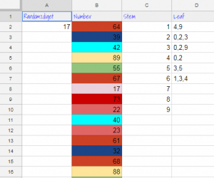
 Fifth graders at Varina Elementary have been learning how to find the mean, median, mode, and range of a set of data (SOL5.16c). They have also been making stem-and-leaf plots (SOL5.15). Today students in Ms. Primrose’s class discovered how to accomplish these tasks using a Google spreadsheet. First, we opened a blank spreadsheet by clicking the shortcut button (the 9-squares at the top of a Google search page). We discussed how the spreadsheet grid is similar to a map grid, with letters along the top and numbers along the side. Each cell has a name based on its letter and number (such as B6 or D9). The cell name stays the same, even if the data inside it changes. I explained that we will be using the cell names to create our formulas for mean, median, mode, and range. This concept of cell names is a great way to help students understand variables (SOL5.18a). Next, we labeled each column: Random, Number, Stem, Leaf, Mean, Median, Mode, Range. I showed them how they could highlight the whole row by clicking 1 on the side and change the font, size, and color. We clicked in A2 and typed our first formula for generating a random 2-digit number: =RANDBETWEEN(10,99). Then we clicked in B2 and typed the number we saw in A2. When we pressed the Enter key we went down to B3 and typed the new random number we saw in A2. We continued doing that until we had about 20 random numbers down column B. To make it easier to create the stem-and-leaf plot, we added some conditional formatting to column B (highlight the column by clicking the B at the top, then click Format > Conditional formatting). We added 9 rules making the cell a different color if the number was between two tens (for example, make the cell red if the value is between 20-29). Now we clicked in the C column (Stem) and typed 1-9 down the cells for our stems. Since the leaves had to be next to the stems, we highlighted the D column (Leaf) and changed the alignment from right to left using the Horizontal align button at the top. Then we used our colors to help us count and enter the numbers. Finally, we used formulas to calculate the mean, median, mode and range in their respective columns:
=AVERAGE(B2:B21)
=MEDIAN(B2:B21)
=MODE(B2:B21)
=MAX(B2:B21)-MIN(B2:B21)
To show the value of using variables (cell names, like B2), I instructed the students to change some of the numbers in Column B. The formulas instantly recalculated their values! We shared our spreadsheets with each other on Schoology, and you can see them all here.

